Bitcoin’s natural long-term power-law corridor of growth
| Crypto Words has moved! The project has migrated to a new domain. All future development will be at WORDS. | Go to WORDS |
Bitcoin’s natural long-term power-law corridor of growth
By Harold Christopher Burger
Posted September 4, 2019
Disclaimer: This article is not financial advice.
With growing adoption of the cryptocurrency, its future price has been the subject of more and more speculation. Predictions are all over the board, with some economists like Nouriel Roubini predicting a price of 0 within five years, whereas John McAfee has famously predicted a price of $1 million per bitcoin by the end of 2020. Others have made predictions that fall within this very wide range [1].
Overall, bitcoin’s price has risen very quickly since it’s initial inception in 2009 and has also been subject to booms and busts. The rapid rises and boom phases seem to encourage people like McAfee to make very optimistic predictions about the future price, whereas the busts seem to encourage some economists to predict a decline toward 0. In this article we look at the full price history of bitcoin and see that bitcoin’s price evolution can be understood as moving within a corridor which is defined by two power-laws based on time. While the idea of modelling bitcoin’s price using a power-law is not new, in this article we give more support to this idea and provide some additional interpretations.

This model allows us to make broad predictions concerning the long-term future price of bitcoin, e.g.
- the price will reach $100 000 per bitcoin no earlier than 2021 and no later than 2028. After 2028, the price will never drop below $100 000.
- the price will reach $1 000 000 per bitcoin no earlier than 2028 and no later than 2037. After 2037, the price will never drop below $1 000 000.
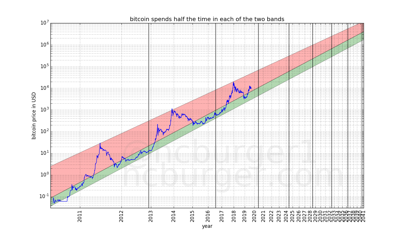
Furthermore, we will see that the price corridor can be divided into two bands, one which lies at the lower-end of the price predictions and is rather thin, the other one being much larger and lying at the higher-end predictions. Bitcoin’s price spends about equal amounts of time in both bands. This implies that large bubbles and busts are likely to continue to exist. The above predictions might seem very broad, but they are sufficiently precise to disagree with the predictions of some other people. This price model should also help determine good points to enter or leave the market.
I am quite confident that in the long-term, the price will indeed evolve approximately as stated in this article. In fact, I think it is more likely for these predictions to be too low rather than too high: I believe that bitcoin has more potential upside than downside to large exogenous shocks. But this article will not try to make any predictions regarding large exogenous shocks. Instead, we will assume that things continue “as usual”.
Different ways of looking at the price
The most interesting and amazing aspect of the price of bitcoin is that it went through many orders of magnitude within a few years. The first instance of a publicly listed price I could find was $0.05 per bitcoin on the Mt Gox exchange, on 17th of July 2010, but prior to that date, many bitcoins have changed hands for a much lower price, such May 22, 2010, when Laszlo Hanyecz paid 10 000 btc for two pizzas, which roughly corresponds to a price of only $0.0025 (0.25 cents) per bitcoin. At the time of writing, the price of one bitcoin hovers around $10 000, which is about 4 million times more than the price at which Laszlo Hanyecz valued them at the time.
Going through so many orders of magnitude is unusual for a financial instrument, and indeed looking at at plot of the price of bitcoin over time might be somewhat confusing (if the price is represented in linear scale). The below is a chart of the price of bitcoin going from the 17th of July 2010 to approximately the time of writing. Similar plots can be found at any website which lists the price of bitcoin.

Any price swings close to the present are so large in magnitude compared to the price in the past, that past prices seem meaningless. However, to make sense of a long-term price trend, all past prices should have some importance. The reason for the above effect is that using a linear scale is inconvenient for anything that goes through so many orders of magnitude. Using a logarithmic rather than linear scale is more useful [2]. The logarithmic scale gives equal spacing from e.g. 0.01 to 0.1 as from 1000 to 10000. Seen in this way, the bigger picture of the price evolution of bitcoin becomes more visible:
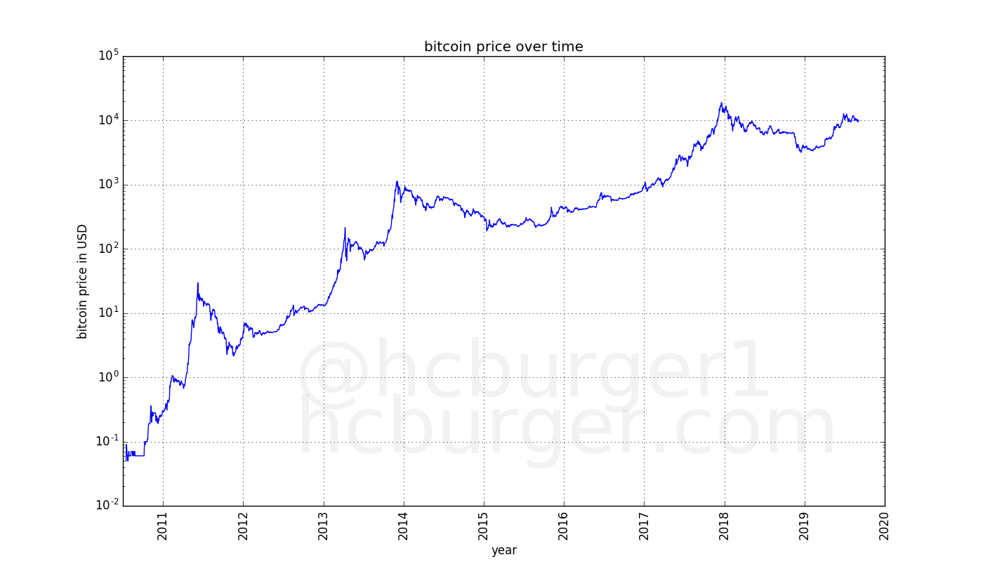
What becomes apparent is that the rate of growth of the price of bitcoin seems to be slowing. The price went from $0.1 to $1 — a factor of 10 — in only a few months. Subsequent gains of a factor 10 came slower.
In the above plot, the price (y-axis) has been scaled logarithmically, but not the time (x-axis). Let’s see what happens when the x-axis is also scaled logarithmically, in a so-called log-log plot [3]:
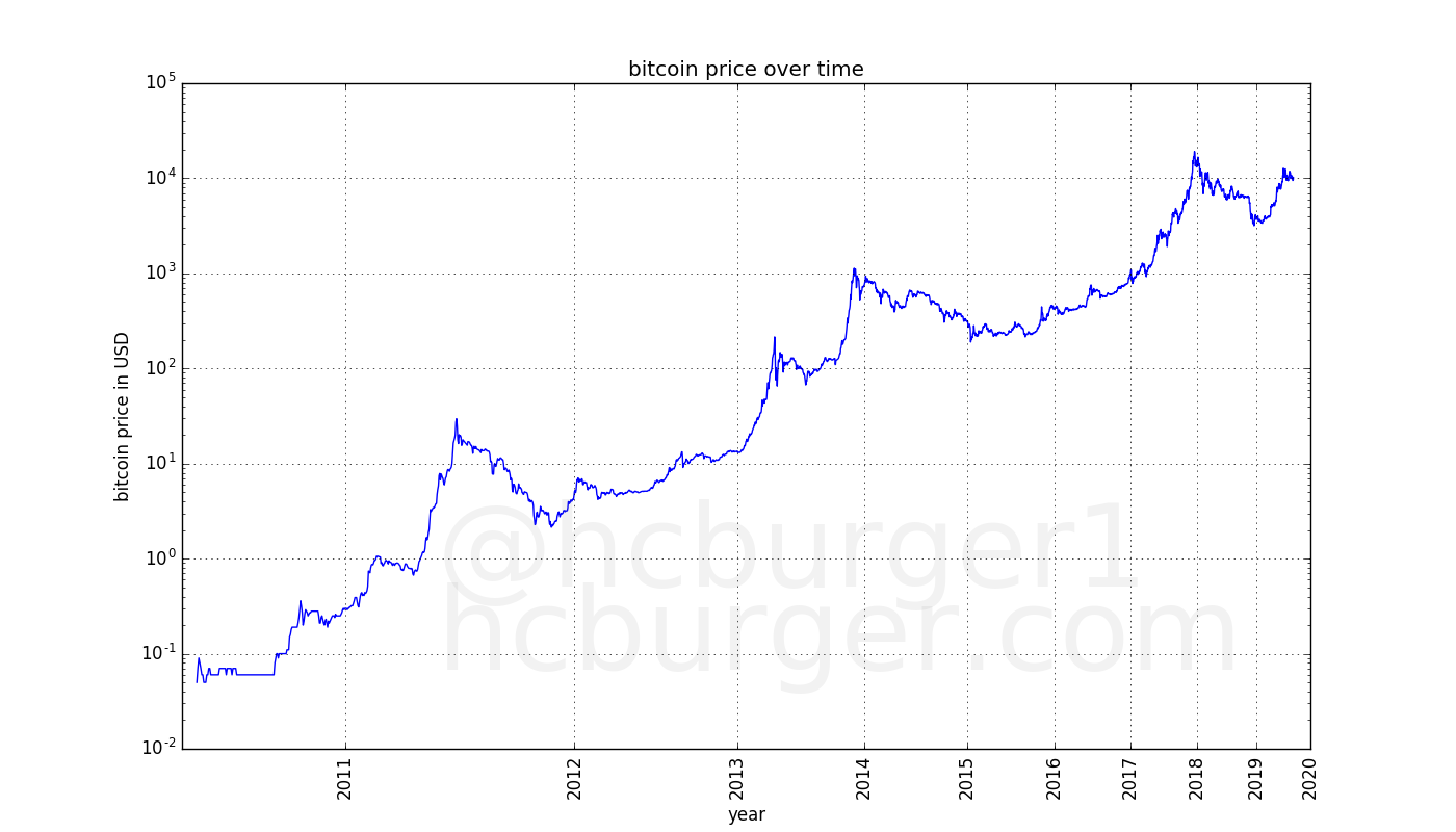
Now the price curve looks remarkably linear!
Linear regression
Since this data looks so linear, let’s try to use linear regression on it [4]. This idea in itself is not new, e.g. I found a post on reddit which did exactly this [5].
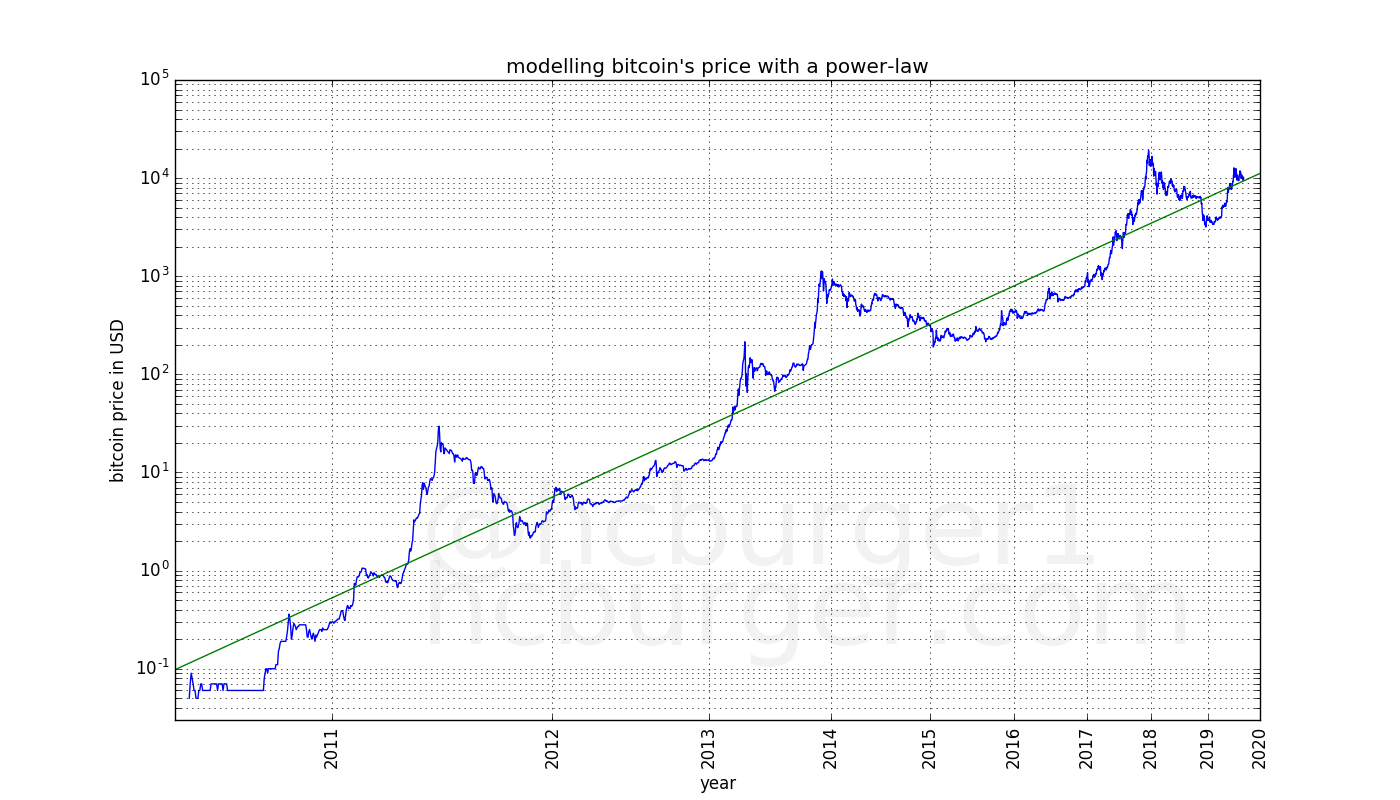
The green line is the result of linear regression. Linear regression gives us the following power-law to predict the price of bitcoin on a given day:

with a = -17.01593313 and the slope b = 5.84509376 with d the number of days since 2009.
Note: We obtain a power-law, which is non-linear because we did linear regression in log-space.
Visually, this fit works very well. It works well all the way back to the first prices that were listed by exchanges. Interestingly, the post on reddit was written about a year ago, and the results are still remarkably similar. Also, the coefficient of determination is high: 0.93139763, which gives us another indication that we have a good model fit [6]. We can look at how the coefficient of determination evolved over time. Surprisingly, the model tends to fit the data better as time goes by:
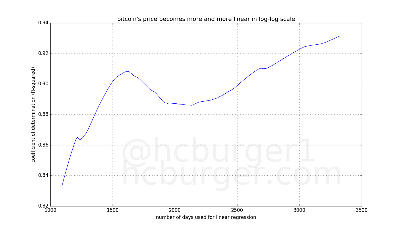
The x-axis represents the number of data points (days) used for the linear regression model, whereas the y-axis represents as a measure of goodness of fit. Bitcoin’s price fits the power-law better and better.
Let’s play around a bit more. If we move the above fit a bit lower (but do not change the slope), we find a support line which seems to work remarkably well: Except for one instance in 2010, the price has never breached this line:
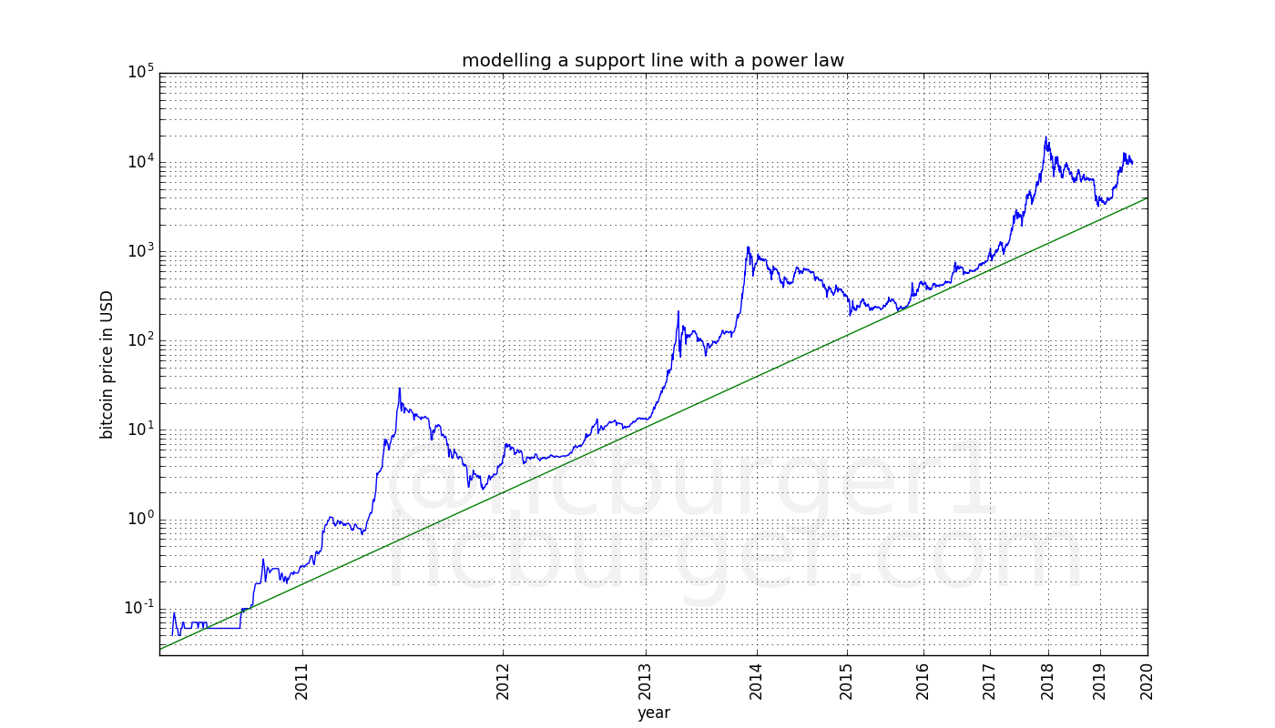
There seems to be a fundamental level of support for bitcoin’s price which has historically followed a power-law.
We can also try to perform linear regression on only the three tops achieved in 2011, 2013, and 2017. Interestingly, this fit works very well: All three data-points are remarkably close to the line:
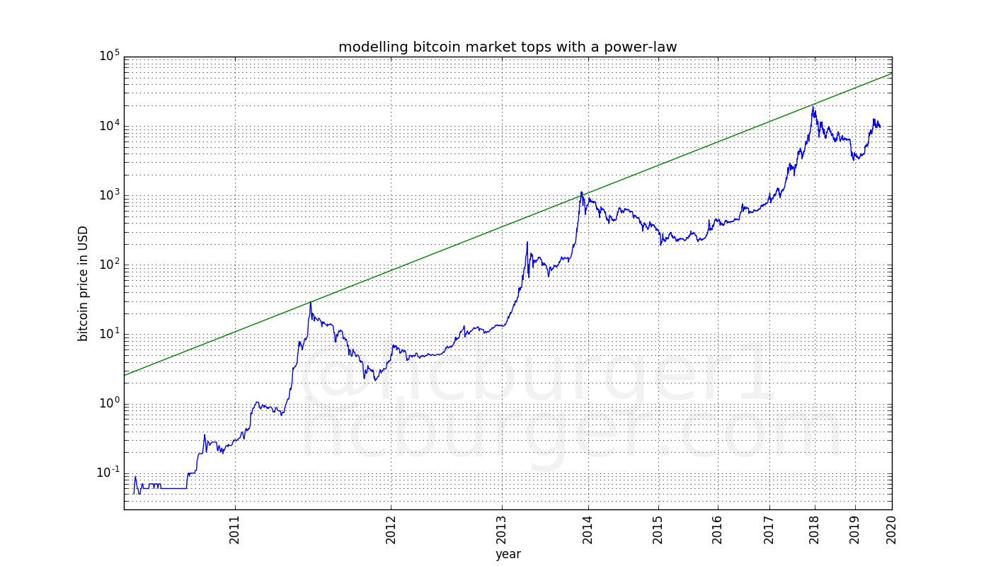
The market tops also seem to follow a power-law. If the next market top also follows this power-law, the market top will lie on this line. The slope of this power-law is 5.02927337, whereas the fit on all data gave us a somewhat larger slope of 5.84509376. This indicates a relative taming of bitcoin bull markets compared to the overall trend-line. This is perhaps expected, as the market matures and order books become deeper, one should expect less volatility.
We now have two power-laws between which the price of bitcoin moves: the lower support line, and the higher line defined by the three market tops.
Now, let’s see which data points fit the model best. We are going to use random sample consensus, or RANSAC, which is an iterative form of outlier removal: First, linear regression is performed on all data points. Then, the data point which fits the data least well is removed, and linear regression is performed again [7]. We’re going to stop when 50% of the data points have been removed. This plot shows the result:
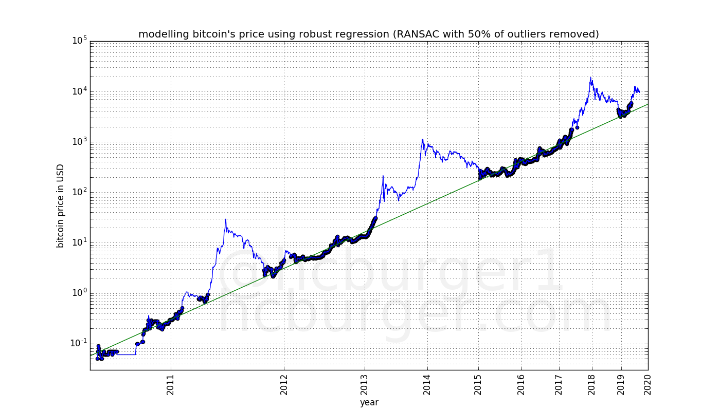
The data points that have been chosen by RANSAC are highlighted in this graph. It seems that there are two groups of data-points: Those that have been chosen by RANSAC are very close to the model fit. In the group of data points not chosen by RANSAC, the values are almost all above the model fit. In fact, some of them are much higher than the model fit. These data-points occurred mostly in bull markets. The price of bitcoin seems to follow two modes:
- the normal mode, during which the price is very well defined by a power law, and
- the bull mode, during which the price can be much higher than in normal mode and during which there is more price volatility.
The price spends equal amounts of time in each of the two modes.
Finally, let’s combine all the previously mentioned model fits into one graph:
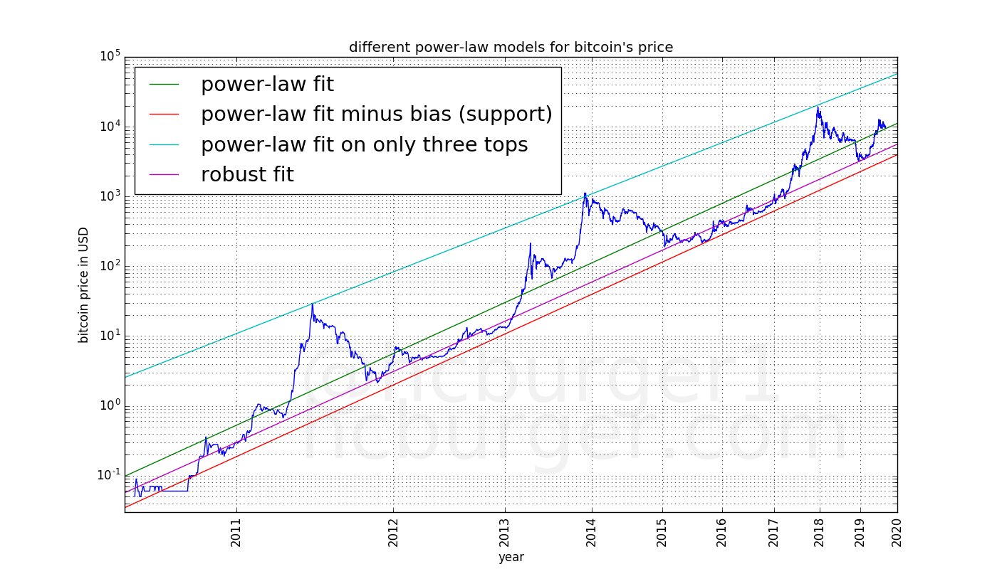
We see that the fit using all data and the result of RANSAC have very similar slope, but a slightly different offset. This is because the bull market prices have been mostly excluded as outliers by RANSAC.
Model predictions
We now have various models to predict the future price of bitcoin. All we have to do is extend the graph:
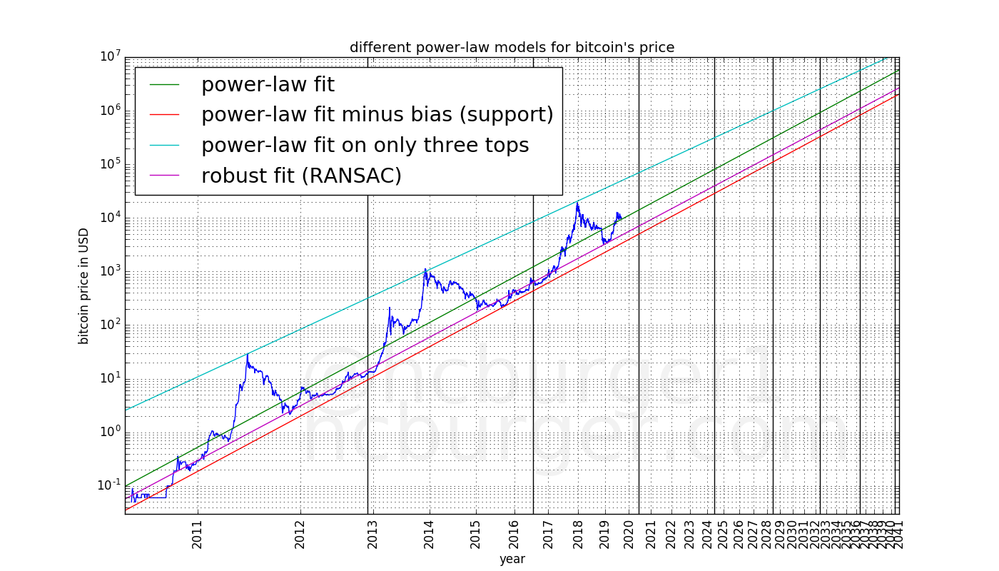
The model predicts that the price will move between the red support line and the blue top line. The purple robust fit / RANSAC line defines the center of the “normal mode”. The two past halvings as well as estimated future halvings have been marked with black vertical lines.
We can further divide this corridor into two bands, one corresponding to the “normal” mode and one corresponding to the “bull” mode. The price has so far spent half the time in the lower “normal mode” band, and the rest of the time in the higher “bull mode” band.
Interpretations
This power-law model predicts a continued, but slowing growth of the price of bitcoin. It also predicts reduced, but still large volatility in the future. It predicts that the price will not reach $100 000 before 2021, but it also predicts that the price will not be lower than $100 000 by 2028. It predicts that the price will not reach $1 000 000 before 2028, but also that the price will not be lower than that after 2037. The model predicts ever increasing prices, although at a slower and slower rate.
These predictions appear to be somewhat middle-of-the-road compared to other predictions. According to this model, McAfee’s famous prediction is far too optimistic.
The combination of the fact that the price corridor is rather wide combined with the fact that the rate of growth is slowing means that unlucky investors will have to wait longer and longer before their initial investment is safely recouped. E.g. investors who bought bitcoin at the top of the bubble in 2011 only had to wait about two years until 2013 for the price of bitcoin to recover permanently. However, investors who bought at the peak of the 2013 bubble had to wait about four years, until 2017, before the price recovered from that price and stayed above that price. The model predicts that the price point reached at the peak of the 2017 bubble might not be secured until the end of 2023, about six years later.
Until now, each four-year halving period had a bubble whose price was exceeded by the next period’s bubble. Due to the above point of slowing growth and corridor width, this is not guaranteed to continue to be the case in the future. As an example, the model allows the following scenario:
- A price of about $150 000 at the beginning of 2022, which is the next and fourth four-year period.
- A price that is lower than $150 000 until mid-2028, which is in the sixth four-year period.
Such a scenario would give bitcoin detractors ammunition for criticism, but is otherwise not something that should be especially worrisome, as long as one is prepared.
Why does bitcoin follow a power-law, and should we expect it to continue? The observation that bitcoin follows a power-law is admittedly ad-hoc. In addition, there are other factors than just time that should influence bitcoin’s price, such as its scarcity. However, bitcoin’s scarcity is programmatic and therefore also time-based. In is therefore not implausible for a simple time-based model to continue to hold true in the future. The fact that the power-law fit works better and better in terms of the measure in the log-log plot is an indication that this might indeed hold.
Conclusion
In this article we presented a simple time-based equations to model bitcoin’s price. It is remarkable that the equations are both 1. simple and 2. use time as the only variable, yet work remarkably well over a long period of time.
This model does not attempt to predict bull markets, which seem to occur periodically. However, bull markets are expected to fall within the corridor defined by this model.
In an upcoming article, we will use a time-based power-law to attempt to find good points in time to enter and exit the market.
References
- https://blockonomi.com/bitcoin-price-predictions-2019/
- https://en.wikipedia.org/wiki/Logarithmic_scale
- https://en.wikipedia.org/wiki/Log%E2%80%93log_plot
- https://en.wikipedia.org/wiki/Linear_regression
- https://www.reddit.com/r/Bitcoin/comments/9cqi0k/bitcoin_power_law_over_10_year_period_all_the_way/
- https://en.wikipedia.org/wiki/Coefficient_of_determination
- https://en.wikipedia.org/wiki/Random_sample_consensus